Local OOR detection

In this tutorial, we will go through the methods for local OOR detection. We recommend that users first read the Introduction to Global and Local OOR Detection section and then choose the method that best suits their needs. Here, we use a preprocessed pseudo-disease dataset as an example.

## load epipack package

# !pip install --upgrade epipackpy
import scanpy as sc
import numpy as np
import pandas as pd

import epipackpy as epk
print(epk.__version__)

1.0.1dev4

import seaborn as sns
import warnings

warnings.filterwarnings("ignore")

sc.set_figure_params(figsize=(6, 6), frameon=False)
sns.set_theme()

Load the simulated data.

A_sim_ = sc.read_h5ad("Fig5_experiment/pbmc_local_oor_detection_result.h5ad")

Please make sure your data also include an obs column named “dataset_group”, in which it contains “query” and “atlas” labels. This can be easily added by using

REF_DATASET.obs['dataset_group'] = 'atlas'
QUUERY_DATASET.obs['dataset_group'] = 'query'

before integration with the query.

#dataset.obs['dataset_group']
A_sim_.obs['dataset_group']

AAACGAAAGACGTCAG-1    query
AAACGAAAGATTGACA-1    query
AAACGAAAGGGTCCCT-1    query
AAACGAACAATTGTGC-1    query
AAACGAACACTCGTGG-1    query
                      ...
TTTGTGTTCGGTACGC-1    atlas
TTTGTGTTCTAATCCT-1    atlas
TTTGTTGGTAAGGTTT-1    atlas
TTTGTTGGTTAGGATT-1    atlas
TTTGTTGGTTTGGGCG-1    atlas
Name: dataset_group, Length: 33307, dtype: category
Categories (2, object): ['atlas', 'query']

Here we first visualization our simulated dataset. The OOR state shows the simulated local OOR cells. Please see our paper for data simulation method.

sc.pp.neighbors(A_sim_, n_neighbors=50, use_rep='z_ref')
sc.tl.umap(A_sim_)
#sc.tl.leiden(tmp, resolution=1.5)
sc.pl.umap(A_sim_, color=['cell_type_new', 'batch_id',"OOR_state"], ncols=2, wspace=0.6)

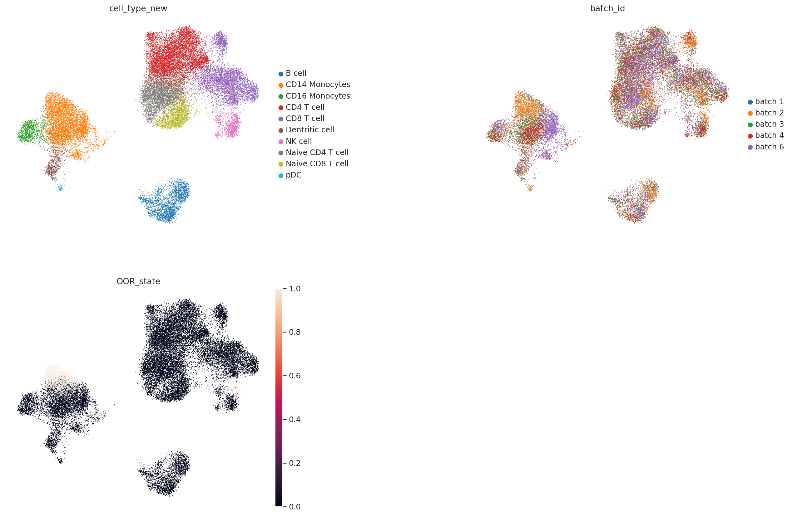
Here we can find that CD14 Monocytes and NK cells both include simulated OOR shifted cell states (batch 1 and 2 are query). Next, we train the local OOR detector.

Z = A_sim_.obsm['z_ref']
y = (A_sim_.obs['dataset_group'].values == 'query').astype(int)
batches = A_sim_.obs['batch_id'].values

res = epk.ml.local_oor_detector(
    Z, y, batches,
    k=30,
    T=20, seed=2048
)

- Constructing edge features...
- Training kernel on cuda (fp32) ...

Epochs: 100%|██████████| 50/50 [00:30<00:00,  1.64it/s, kernel_converge_loss=0.127]

- Running BRP on the graph...
- FDR control with significance value  0.1 ...
- Done!

Res dataframe contains all result related to the detection result. Some of those useful terms as listed below:

• K is the trained kernel

• prob is the probability that this cell belongs to the query setting (experimental group)

• qval is significant value after FDR control

• significant is the binary result of the detected OOR cells

A_sim_.obs['OOR_prob']  = res['prob']
A_sim_.obs['OOR_pval']  = res['pval']
A_sim_.obs['OOR_qval']  = res['qval']
A_sim_.obs['OOR_sig_predicted']  = res['significant'].astype(int)

We visualize the probability and q value below. For CD14 Monocytes, we have

mask = (A_sim_.obs['cell_type_new'] == 'CD14 Monocytes').values
Z_sub = Z[mask]; y_sub = y[mask]; batches_sub = batches[mask]

sc.pl.umap(A_sim_[mask], color=['OOR_prob', "OOR_qval"], ncols=2, wspace=0.6)

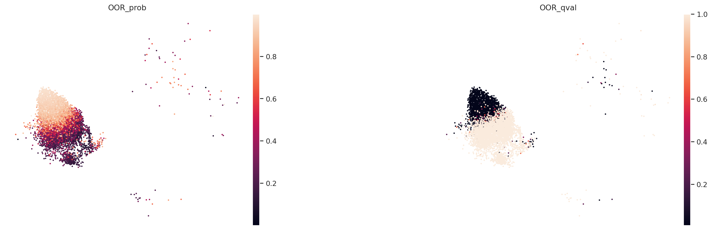
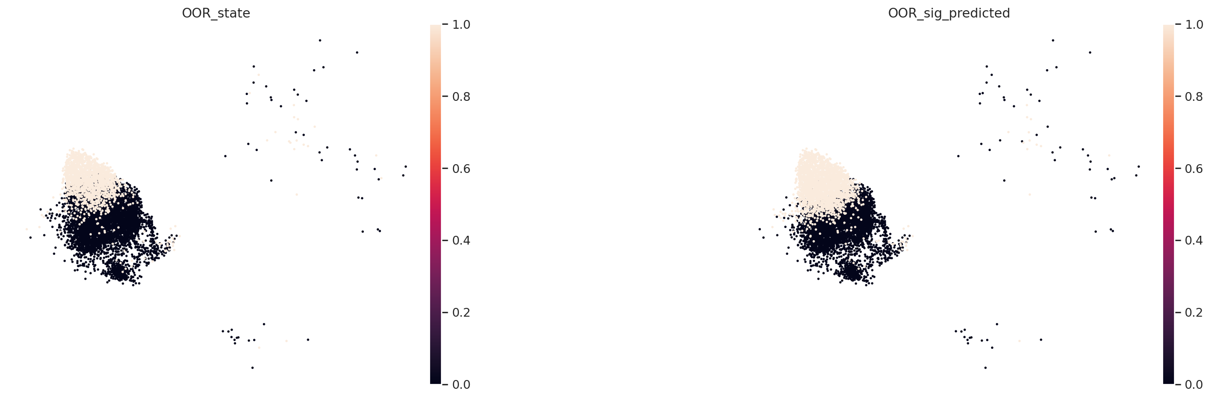
We can find that our predicted local OOR cell states is largely overlapped with the ground truth OOR state label.

sc.pl.umap(A_sim_[mask], color=['OOR_state','OOR_sig_predicted'], ncols=2, wspace=0.6)

We can also calculate enrichment score.

# calculate enrichment score
eps = 1e-5
p = A_sim_.obs["OOR_prob"].clip(eps, 1-eps).to_numpy()
A_sim_.obs["enrichment_score"] = np.log10(p/(1-p))

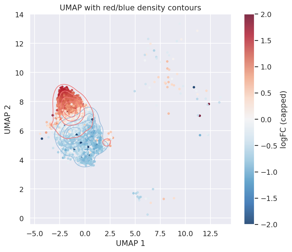
We visualize CD14 Monocyte enrichment score density map below.

umap_ = pd.DataFrame(A_sim_[mask].obsm['X_umap'],   columns=['UMAP1', 'UMAP2'])
umap_['logfc_cap'] = (
    A_sim_[mask].obs["enrichment_score"].to_numpy().clip(-2, 2)
)

#import pandas as pd
import matplotlib.pyplot as plt
#import seaborn as sns
#import numpy as np

plt.figure(figsize=(7,6))
sc = plt.scatter(
    umap_["UMAP1"],
    umap_["UMAP2"],
    c=umap_["logfc_cap"],
    cmap="RdBu_r", vmin=-2, vmax=2,
    s=8, alpha=0.8
)

sns.kdeplot(
    data=umap_[umap_["logfc_cap"] < 0],
    x="UMAP1", y="UMAP2",
    levels=5,  color="#99bcdc", linewidths=1
)

sns.kdeplot(
    data=umap_[umap_["logfc_cap"] > 0],
    x="UMAP1", y="UMAP2",
    levels=5, color="#f0797a", linewidths=1
)

plt.colorbar(sc, label="logFC (capped)")
plt.xlabel("UMAP 1")
plt.ylabel("UMAP 2")
plt.title("UMAP with red/blue density contours")
plt.show()